The R class R programming for biologists
02 -- coercion, lists, factors, and a little bit of `data.frame`
Coercion
Last week, we covered vectors. Vectors are data structures that R uses to store information. We spent some time covering how vectors have classes associated with them. What happens if we try to create a vector that contains elements of different classes?
x <- c(123, "cats", TRUE)
class(x)
## [1] "character"
What happened here? Vectors can only have 1 class associated with them, therefore R has to make decisions to convert (= coerce) the content of this vector to find a “common denominator”. To figure out the rules R uses let’s explore some options:
class(c(TRUE, 1))
## [1] "numeric"
class(c(TRUE, "cats"))
## [1] "character"
class(c(1, "cats"))
## [1] "character"
logical --> numeric --> character <-- logical
These conversions between formats can even be used to do maths:
1 + TRUE # TRUE == 1
## [1] 2
1 + FALSE # FALSE == 0
## [1] 1
and vectors of logicals can be used with functions normally used with numbers:
## Gives the number of elements that are TRUE
sum(c(TRUE, FALSE, TRUE, TRUE, FALSE, TRUE))
## [1] 4
## Gives the proportion of elements that are TRUE
mean(c(TRUE, FALSE, TRUE, TRUE, FALSE, TRUE))
## [1] 0.6666667
These properties are really useful in conjunction with tests as we saw last week.
x <- 0:100
x < 40
##   [1]  TRUE  TRUE  TRUE  TRUE  TRUE  TRUE  TRUE  TRUE  TRUE  TRUE  TRUE
##  [12]  TRUE  TRUE  TRUE  TRUE  TRUE  TRUE  TRUE  TRUE  TRUE  TRUE  TRUE
##  [23]  TRUE  TRUE  TRUE  TRUE  TRUE  TRUE  TRUE  TRUE  TRUE  TRUE  TRUE
##  [34]  TRUE  TRUE  TRUE  TRUE  TRUE  TRUE  TRUE FALSE FALSE FALSE FALSE
##  [45] FALSE FALSE FALSE FALSE FALSE FALSE FALSE FALSE FALSE FALSE FALSE
##  [56] FALSE FALSE FALSE FALSE FALSE FALSE FALSE FALSE FALSE FALSE FALSE
##  [67] FALSE FALSE FALSE FALSE FALSE FALSE FALSE FALSE FALSE FALSE FALSE
##  [78] FALSE FALSE FALSE FALSE FALSE FALSE FALSE FALSE FALSE FALSE FALSE
##  [89] FALSE FALSE FALSE FALSE FALSE FALSE FALSE FALSE FALSE FALSE FALSE
## [100] FALSE FALSE
sum(x < 40)
## [1] 40
This is a really R way of doing things that we will take advantage of when we’ll be writing functions.
Lists
Lists are an extension of vectors that allow the storage of multiple classes in a single object.
x <- list(123, "cats", TRUE)
class(x)
## [1] "list"
x
## [[1]]
## [1] 123
##
## [[2]]
## [1] "cats"
##
## [[3]]
## [1] TRUE
- Show how R presents lists, the double [[]] and the single [].*
We can use [[]] to select each element of the list:
x[[1]]
## [1] 123
class(x[[1]])
## [1] "numeric"
Lists can contain vectors of different lengths:
x <- list(c(5, 10, 20), "cats", c(TRUE, FALSE))
x[[1]]
## [1] 5 10 20
x[[1]][2]
## [1] 10
Similarly to vectors, lists can be nammed:
x <- list("numbers"=c("first"=5, "second"=10, "third"=20),
          "animals"=c("cats", "dogs", "chickens"),
          "logicals"=c(TRUE, FALSE, TRUE))
x[[2]][1]
## [1] "cats"
x["animals"][1]
## $animals
## [1] "cats"     "dogs"     "chickens"
x$animals[1]
## [1] "cats"
names(x)
## [1] "numbers" "animals" "logicals"
Challenge
How can you obtain the name of the second element inside the vector contained in
the first item in this list? In other words, what is the command that would
return "second"?
Answer
Possible answers:
names(x$numbers)[2]
names(x$numbers[2])
names(x[[1]][2])
Presentation of the Survey Data
We are studying the species and weight of animals caught in plots in our study
area. The dataset is stored as a .csv file: each row holds information for a
single animal, and the columns represent survey_id , month, day, year,
plot, species (a 2 letter code, see the species.csv file for
correspondance), sex (“M” for males and “F” for females), wgt (the weight in
grams).
The first few rows of the survey dataset look like this:
"63","8","19","1977","3","DM","M","40"
"64","8","19","1977","7","DM","M","48"
"65","8","19","1977","4","DM","F","29"
"66","8","19","1977","4","DM","F","46"
"67","8","19","1977","7","DM","M","36"
To load our survey data, we need to locate the surveys.csv file. We will use
read.csv() to load into memory (as a data.frame) the content of the CSV
file.
download.file("http://r-bio.github.io/data/surveys.csv", "data/surveys.csv")
surveys <- read.csv('data/surveys.csv')
This statement doesn’t produce any output because assignment doesn’t display
anything. If we want to check that our data has been loaded, we can print the
variable’s value: surveys
Wow… that was a lot of output. At least it means the data loaded
properly. Let’s check the top (the first 6 lines) of this data.frame using the
function head():
head(surveys)
##   record_id month day year plot species sex wgt
## 1         1     7  16 1977    2      NL   M  NA
## 2         2     7  16 1977    3      NL   M  NA
## 3         3     7  16 1977    2      DM   F  NA
## 4         4     7  16 1977    7      DM   M  NA
## 5         5     7  16 1977    3      DM   M  NA
## 6         6     7  16 1977    1      PF   M  NA
Let’s now check the __str__ucture of this data.frame in more details with the
function str():
str(surveys)
## 'data.frame':	35549 obs. of  8 variables:
##  $ record_id: int  1 2 3 4 5 6 7 8 9 10 ...
##  $ month    : int  7 7 7 7 7 7 7 7 7 7 ...
##  $ day      : int  16 16 16 16 16 16 16 16 16 16 ...
##  $ year     : int  1977 1977 1977 1977 1977 1977 1977 1977 1977 1977 ...
##  $ plot     : int  2 3 2 7 3 1 2 1 1 6 ...
##  $ species  : Factor w/ 49 levels "","AB","AH","AS",..: 17 17 13 13 13 24 23 13 13 24 ...
##  $ sex      : Factor w/ 6 levels "","F","M","P",..: 3 3 2 3 3 3 2 3 2 2 ...
##  $ wgt      : int  NA NA NA NA NA NA NA NA NA NA ...
Also, show how to get this information from the “Environment” tab in RStudio.
Challenge
Based on the output of str(surveys), can you answer the following questions?
- What is the class of the object
surveys? - How many rows and how many columns are in this object?
- How many species have been recorded during these surveys?
As you can see, the columns species and sex are of a special class called
factor. Before we learn more about the data.frame class, we are going to
talk about factors. They are very useful but not necessarily intuitive, and
therefore require some attention.
Factors
Factors are used to represent categorical data. Factors can be ordered or unordered and are an important class for statistical analysis and for plotting.
Factors are stored as integers, and have labels associated with these unique integers. While factors look (and often behave) like character vectors, they are actually integers under the hood, and you need to be careful when treating them like strings.
Once created, factors can only contain a pre-defined set values, known as levels. By default, R always sorts levels in alphabetical order. For instance, if you have a factor with 2 levels:
sex <- factor(c("male", "female", "female", "male"))
R will assign 1 to the level "female" and 2 to the level "male" (because
f comes before m, even though the first element in this vector is
"male"). You can check this by using the function levels(), and check the
number of levels using nlevels():
levels(sex)
## [1] "female" "male"
nlevels(sex)
## [1] 2
Sometimes, the order of the factors does not matter, other times you might want to specify the order because it is meaningful (e.g., “low”, “medium”, “high”) or it is required by particular type of analysis. Additionally, specifying the order of the levels allows to compare levels:
food <- factor(c("low", "high", "medium", "high", "low", "medium", "high"))
levels(food)
## [1] "high" "low" "medium"
food <- factor(food, levels=c("low", "medium", "high"))
levels(food)
## [1] "low" "medium" "high"
min(food) ## doesn't work
## Error in Summary.factor(structure(c(1L, 3L, 2L, 3L, 1L, 2L, 3L), .Label = c("low", : 'min' not meaningful for factors
food <- factor(food, levels=c("low", "medium", "high"), ordered=TRUE)
levels(food)
## [1] "low" "medium" "high"
min(food) ## works!
## [1] low
## Levels: low < medium < high
In R’s memory, these factors are represented by numbers (1, 2, 3). They are
better than using simple integer labels because factors are self describing:
"low", "medium", and "high"” is more descriptive than 1, 2, 3. Which
is low? You wouldn’t be able to tell with just integer data. Factors have this
information built in. It is particularly helpful when there are many levels
(like the species in our example data set).
Converting factors
If you need to convert a factor to a character vector, simply use
as.character(x).
Converting a factor to a numeric vector is however a little trickier, and you have to go via a character vector. Compare:
f <- factor(c(1, 5, 10, 2))
as.numeric(f)               ## wrong! and there is no warning...
## [1] 1 3 4 2
as.numeric(as.character(f)) ## works...
## [1] 1 5 10 2
as.numeric(levels(f))[f] ## The recommended way.
## [1] 1 5 10 2
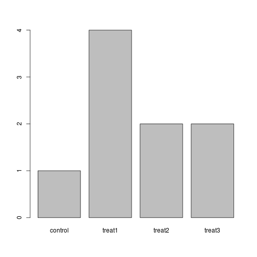
Challenge
The function table() tabulates observations and can be used to create
bar plots quickly. For instance:
## Question: How can you recreate this plot but by having "control"
## being listed last instead of first?
exprmt <- factor(c("treat1", "treat2", "treat1", "treat3", "treat1", "control",
                   "treat1", "treat2", "treat3"))
table(exprmt)
## exprmt
## control  treat1  treat2  treat3
##       1       4       2       2
barplot(table(exprmt))